Counting items in warehouse bins on AWS SageMaker

Fulfillment centers move enormous numbers of products, and every bin that leaves a shelf should hold the right number of items. Amazon released the Amazon Bin Image Dataset (ABID) with a set of challenge tasks around this problem. This project tackles one of them, counting the objects in a bin from a single photo, and asks whether replacing the baseline model's head with more expressive architectures improves the count.

Code, notebook and results: carlos-dev-research/aws-abid-count-task.

A bin from the dataset: items partly hidden behind the elastic bands that hold them in place

The photo above shows why this is hard. Items overlap, sit behind elastic retaining bands, and vary from small pouches to large boxes.

The data#

ABID contains over 500,000 bin photos, each with metadata listing the items inside. I streamed images directly from the public aft-vbi-pds S3 bucket and resized them to 3×224×224.

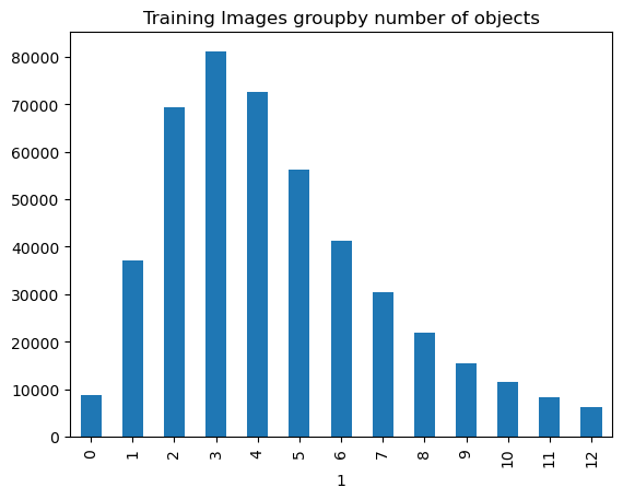
Number of training images per object count: most bins hold 2 to 5 items, and few hold 10 or more

The counts are heavily skewed. I kept bins with 0 to 12 items, which covers about 95% of the data, giving 13 classes. To keep costs manageable and avoid the model simply learning the most common counts, I built a balanced subset of about 1% of the dataset:

Split	Per count	Total
Training	400	5,200
Validation	80	1,040

Each batch held 13 images, one per count. While setting up training I found that some indexed images no longer existed in the bucket, so I rebuilt the lists from verified images while keeping the same per-count balance.

Four heads on one backbone#

The challenge's reference solution is a ResNet-34 with a dense classification layer, trained on bins with 0 to 5 items. I started from its pretrained weights, froze the backbone, and trained only a new head on top. That isolates the question: can a better head extract a count from the same features?

Head	Idea
`DNN_HEAD`	The baseline: pooled features → linear layer
`CNN_HEAD`	An extra 3×3 convolution before pooling, to learn dataset-specific spatial features
`ATT_HEAD`	Multi-head self-attention across the 7×7 feature map before pooling
`MULTIPLE_CNN_HEAD`	Three parallel convolutions with wide, tall and square kernels, for objects of different shapes

The multi-kernel head, for example:

kernel_sizes = [(9, 19), (19, 9), (9, 9)]
self.convs = nn.ModuleList([
    nn.Conv2d(in_features, 256, kernel_size=k, padding=[ki // 2 for ki in k])
    for k in kernel_sizes
])

def forward(self, x):
    x = self.resnet34(x)
    x = torch.cat([self.relu(conv(x)) for conv in self.convs], dim=1)
    x = self.flatten(self.gap(x))
    return self.Linear(x)

Each head came in two flavours:

Classification: 13 outputs, one per count, trained with cross-entropy.
Regression: one extra linear layer producing a single number, trained with mean squared error and rounded to the nearest count.

Training on SageMaker#

All variants share one training script, train.py. SageMaker's HyperparameterTuner launched every combination of head, output type and learning rate as a separate job: 4 × 2 × 2 = 16 training jobs, each 10 epochs with Adam on an ml.g4dn.xlarge GPU instance.

hyperparameter_ranges = {
    "learning_rate": CategoricalParameter([0.0001, 0.001]),
    "model_name": CategoricalParameter(["DNN_HEAD", "CNN_HEAD", "ATT_HEAD", "MULTIPLE_CNN_HEAD"]),
    "type_of_inference": CategoricalParameter(["linear_regression", "classification"]),
}

Results#

With predictions $p_i$ and true counts $g_i$ over $N$ images:

\text{Accuracy} = \frac{1}{N}\sum_{i=1}^{N} \mathbb{1}[p_i = g_i] \qquad \text{RMSE} = \sqrt{\frac{1}{N}\sum_{i=1}^{N} (p_i - g_i)^2}

Validation results, at the better of the two learning rates for each head (by accuracy):

Head	Output	Val accuracy	Val RMSE	Train accuracy
`DNN_HEAD` (baseline)	classification	8.9%	5.57	11.1%
`CNN_HEAD`	classification	8.7%	5.37	18.9%
`ATT_HEAD`	classification	9.3%	5.14	19.0%
`MULTIPLE_CNN_HEAD`	classification	9.3%	4.91	23.5%
`DNN_HEAD`	regression	8.0%	3.79	7.7%
`CNN_HEAD`	regression	8.3%	3.99	8.9%
`ATT_HEAD`	regression	9.1%	4.78	9.6%
`MULTIPLE_CNN_HEAD`	regression	9.9%	4.13	11.1%

At the time, I read this as two findings. The multi-kernel head had the best accuracy, and the regression heads had a much lower RMSE than classification. A follow-up run of the regression DNN_HEAD for 100 epochs reached 8.6% validation accuracy, barely moving.

Looking back: compare against trivial baselines#

Coming back to these numbers, the right comparison is not between heads but against models that learn nothing:

Random guessing. The validation set is balanced across 13 counts, so guessing gives $1/13 \approx 7.7\%$ accuracy. The best head reaches 9.9%, only about 2 points above chance.
Always predicting the mean. If a model always answers 6, its squared error over a balanced 0–12 set is the variance of that range:

\frac{1}{13}\sum_{k=0}^{12} (k - 6)^2 = \frac{13^2 - 1}{12} = 14 \quad\Rightarrow\quad \text{RMSE} = \sqrt{14} \approx 3.74

Two of the regression runs land on an MSE of exactly 14.00, with accuracy right at chance. They collapsed to predicting a constant. The regression heads' lower RMSE mostly reflects that predicting the middle of the range is a safe bet under squared error, not that they learned to count. Meanwhile, the classification heads reach up to 23.5% on training data but stay near chance on validation, a sign they were memorizing the small training set.

The likely causes:

A frozen backbone trained on a different task. The pretrained features were learned for 0–5 items, but here they had to separate 0–12, and only the head could adapt.
Little data. About 5,200 images, for a task with heavy occlusion and very different item sizes.
Optimization. The reference repository reports much better results with a different optimizer and full training of the network.

Takeaways#

Put trivial baselines in the results table from day one. "Random" and "always predict the mean" would have reframed every comparison immediately.
Architecture changes can't fix features that don't carry the signal. With the backbone frozen, the head choice barely mattered.
Next steps: unfreeze the backbone (at least the last blocks), train on far more of the dataset, and revisit the optimizer and schedule from the reference solution.
SageMaker's tuner made a 16-way experiment a single launch, which is the right setup for running these next experiments.

Resources#

Code and notebook: github.com/carlos-dev-research/aws-abid-count-task
Amazon Bin Image Dataset and its documentation
ABID challenge reference solution